Deep Reinforcement Learning Lab

This lab is about using DRL to solve the CartPole problem (continuous input, discrete actions) using methods inspired by DQN. By running it and changing parameters, we can learn more about the meaning of the key parameters and DRL. This lab is my note after course given by Nicolas HOFFMANN in Telecom-SudParis, at ARTEMIS research group. The implementation code is provided by him.

Before doing this lab, I make an introductory post on the keywords related to Reinforcement Learning.

Deep Network

In classic reinforcement learning, we use a table for agent to note the value (V value or Q value) for a pair of state and action. The tabular method is not useful for this problem because the input is not discrete. When the agent explore it, the value will be updated at the cell. In DRL, the value function will be replaced by a neural network. To specify, the V Neural Network will take a state vector as input, while the Q Neural Network will take a state-action vector as input.

Problem statement

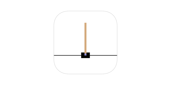
For this lab, we use the Cart Pole problem as demonstration. The black part is the cart which we can move left or right. We should keep the straight not fallen while moving. In order to describe the state, we have 4 numbers: the position and speed for the cart and pole. For Action Space, we have 2 actions: left and right.

Code

The implementation notebook will be worked on Google Colab, with running on GPU. The environment is simulated by using gym package. The detail can be found here.

QNetwork

The QNetwork class defines the Q-value function network with the constructor taking stateSpace, actionSpace, width of network and dropoutRate of neural network as inputs.

class QNetwork(torch.nn.Module):
    def __init__(self, stateSpace, actionSpace, width=64, dropoutRate=0.5):

It also defines function Q which will return the Q-value of a specific action, or all values for all possible actions.

Doer

The Doer class defines how agent acts. The constructor will take the model, stateSpace, actionSpace and epsilon as parameters. The epsilon is the probability of doing random exploration. For example here epsilon=0.1, about 10% of time the agent will explore by acting randomly, and for other time it will evaluate the collected data to find optimal action.

class Doer():
  def __init__(self, model, stateSpace, actionSpace, epsilon=0.1):

Experience Replay

Briefly speaking, experience replay is to record how an agent behaves in a buffer and later evaluate with the data. One of the advantage of it is that we can use efficiently the previous experience, which is useful when the experience gaining is expensive or hard. In code, a Transition class is defined to record the state, action, reward, nextState and nextAction. Relevance denotes the usefulness of a transition object for training the network. The more useful, the more it is relevant.

class Transition():
  def __init__(self, St, At, Rt, Stp, Atp, isTerminal=False, ID=None, relevance=None, birthdate=-1):

The ExperienceReplay class defines the transition storage and usage. The weightedBatches denotes if we use the different weights on transitions based on their relevance. When the sortTransition is activated and when the buffer is full, this class will delete those with least relevance.

class ExperienceReplay():
  def __init__(self, bufferSize=1000, batchSize=256, weightedBatches=True, sortTransition=False):

Learner

The class Learner defines the optimal policy algorithm like SARSA and Q-Learning. One of the parameters here, gamma, denotes the discounted factor.

Firstly, we will have two network, target and frozenTarget, and the latter is a copy of the first one. We will update target and compare it to frozenTarget later.

The difference between SARSA and QLEARNING is the part of target value: SARSA takes directly some next action while QLEARNING takes the optimal action by calculating the maximum size of Q-value. Step by step, the two algorithms try to make the internal target value equals to the Q-value of current transition, by shortening the losses. Once this is done, an episode containing several steps is finished.

An loss value is defined by using MSE method, to know the difference of target value and Q-value of current transition.

After an episode is finished, all the transitions’ relevance will be updated according to the losses calculated before, so that next time, we can use the one with most loss(most relevance) firstly.

   """ Learns from <batch> using algo "SARSA" or "QLEARNING"

    SARSA : Q(St, At) <- Q(St, At) + alpha * [Rt+1 + gamma * Q(St+1, At+1) - Q(St, At)]

    Q-Learning : Q(St, At) <- Q(St, At) + alpha * [Rt+1 + gamma * max(Q(St+1, a)) - Q(St, At)] """

Training loop

The training loop is where training happens. The code are divided into two parts: initialization and looping. As for initialization, we need to create the instance of all building blocks mentioned before. This is where we tune for experimenting. The training loop will continue training if we do not stop it manually. Each 100 iteration, the exploration rate epsilon will change and the frozenTarget will be updated. Once and episode is done, the environment will be reset.

One thing to note is that we can have several ERs here, and in this case the loss will be the average of them. The loss will be noisy because the data will keep changing.

Evaluation

The evaluation code is divided by the graph part and the log of transition data in an episode. For the graph, the reward and score are plotted. The goal of this lab is to modify the parameters and make the score as high as possible. For the log, what interests us will be the rightmost part, where we can see the reward it should have by taking left or taking right.

transition + qValues : [Transition] St: [-0.03888473  0.04604334 -0.01238872 -0.03465939] | At: None | Rt: 1.0 | St+1: [-0.03796386 -0.14889879 -0.01308191  0.25408916] | At+1: 0 | isTerminal: False | ID: None | relevance: None | birthdate: 99 		tensor([[6.4874, 7.1039]], grad_fn=<PermuteBackward>)
transition + qValues : [Transition] St: [-0.03796386 -0.14889879 -0.01308191  0.25408916] | At: 0 | Rt: 1.0 | St+1: [-0.04094184  0.04640749 -0.00800013 -0.04269116] | At+1: 1 | isTerminal: False | ID: None | relevance: None | birthdate: 99 		tensor([[6.5085, 7.1262]], grad_fn=<PermuteBackward>)
transition + qValues : [Transition] St: [-0.04094184  0.04640749 -0.00800013 -0.04269116] | At: 1 | Rt: 1.0 | St+1: [-0.04001369 -0.14859884 -0.00885395  0.24745696] | At+1: 0 | isTerminal: False | ID: None | relevance: None | birthdate: 99 		tensor([[6.4920, 7.1068]], grad_fn=<PermuteBackward>)
transition + qValues : [Transition] St: [-0.04001369 -0.14859884 -0.00885395  0.24745696] | At: 0 | Rt: 1.0 | St+1: [-0.04298567  0.04664844 -0.00390481 -0.0480055 ] | At+1: 1 | isTerminal: False | ID: None | relevance: None | birthdate: 99 		tensor([[6.5087, 7.1265]], grad_fn=<PermuteBackward>)

Key parameters

width

width of neural network. Normally a more complex(big) neural network is suitable for handling complex problem.

optimizer

SGD or Adam

algorithm

sarsa or q-learning

gamma

discounted rate

epsilon

rate for exploring, if set as 1, then it will do randomly

bufferSize

how many transitions can be stored in ER

batchSize

how many transitions will be trained

ER combination

by setting sortTransition and weightedBatches true or false, there will be four combinations and we can use only one or even four together

doer

By setting a doer as random, it will go left or right with one half chance. However, for training, it is not useful because it learns nothing.

Experiments

The first thing I do is try to make the epsilon lower platform value to be 0.3, to explore more in other words. Compared to the case of 0.1, it does more randomly and can rapidly get a score of 25. However it drops rapidly later, because of this random exploration. I reset it as 0.05 and it is close to 10 as score.

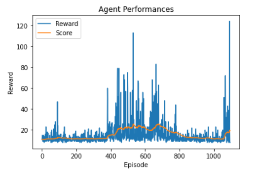
epsilon at 0.3

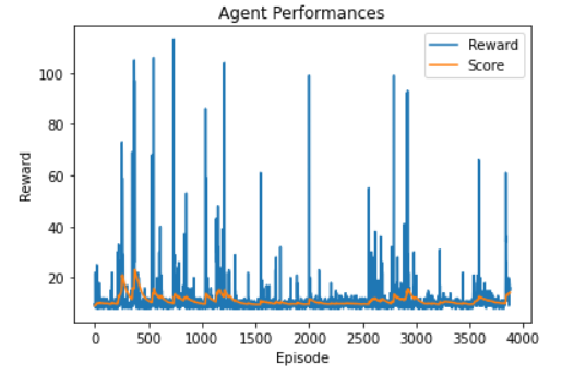
epsilon at 0.05

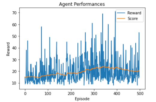
This give me an inspiration to do a high epsilon for the beginning and let cache memorize them by using the relevant sorting and weighted batches. So I set for the first 10,000 iteration a epsilon as 0.5, and after that change it to 0.1. The result is encouraging because the highest score can be 45, with other parameters as default.

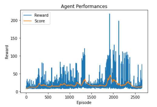
q-Learning, epsilon at 0.5 and later 0.1, with relevanceSorting and weightedBatches true

The next experiment is to add the size so that the complexity of network and buffer size is enough, even it takes longer.

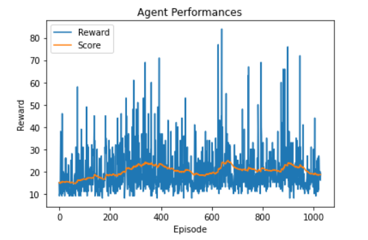
q-Learning, epsilon at 0.5 and later 0.1, with relevanceSorting and weightedBatches true, bufferSize=4096, batchSize=1024, width = 128

The first part with high epsilon rate results in around 25 as score after 10,000 iteration. However, changing it into 0.1 will not help it advance.

The next thing I examine is the gamma, the discounted factor. I change it to be 0.8. The reward gets higher but the scores remain the same, under 20.

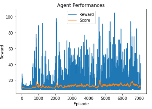
gamma at 0.8

Another test is trying to make the size of buffer and width of network. But the result does not improve too much.

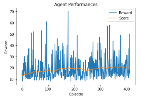
big size in width and bufferSize

The next experiment is to activate four ERs so that each kind of experience will be tested at the same time. The result is at 20 in average.

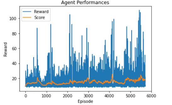
four experience replays

The last experiment is to change the update rate for frozen network, so that a target will change not frequently. From the graph below, it do improve a bit, ranges at 10 to 30.

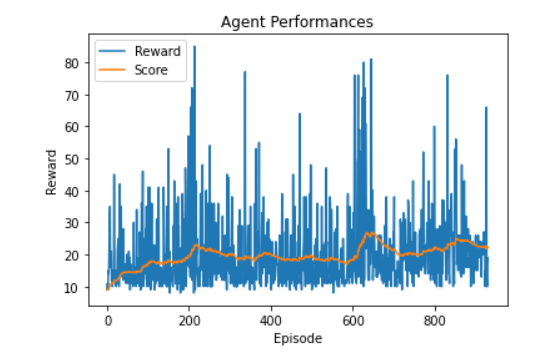
frozen network update after 1000 iteractions, big size of width and buffer size

Conclusion

The theory part of reinforcement learning is interesting, especially the thought of using neural network to replace the table matrix. By imitating the way a human learns thing, RL is very powerful in AI implementation in game. Unlike supervised learning, the unlabelled data makes it harder to train. Understanding the meaning of parameters will help in tuning system. However it is still difficult to connect one observation with the change of a parameter in experiments. What makes this harder is the influence of random seed at initialization.