Basics of RNN
Recurrent neural network is a type of network architecture that accepts variable inputs and variable outputs[1].
Table of contents
In this post I will talk about the fundamental concepts of RNN and its variations like LSTM. This post is my note after course given by Hugo DURCHON in Telecom-SudParis, at ARTEMIS research group. Some of the graphs in this post are from his presentation.
Sequence
Sequential data is everywhere, such as music, video. For definition, a sequence is an enumerated and ordered collection of objects in which repetitions are allowed. The order is crucial for a sequence. In other words, a specific order of elements leads to a specific result.
FeedForward Neural Network
A FeedForward Neural Network involves the neurons whose connections do not form a cycle. Typically FFNN accepts a fixed-size input and give an output. Multi Layer Perceptron is an example of type FFNN.
A natural question is that: can we try to build a FFNN to complete a classification task over a sequence? Let us think about a concrete problem: sentiment analysis. The input should be a sentence and the output should be a classification among positiveness and negativeness.
The first issue that FFNN encounters is the length of input. FFNN requires that the input has the same size, while a sentence can be with different size of words. Even if we make a dictionary of all the positive or negative words and use this one-word to do classification, the result will not be optimal. As we know, we cannot isolate a word from its context. Take an example: “In spite of minor flaws a movie you won’t want to miss”. We, as humans, can know that it is still a good movie. However, the word flow will make this model go into a wrong classification.
Even though we take a several-words size window, we will lose the generalization of this model. Therefore, FFNN is not a good choice for sequence.
Sequence Modeling Problems
In real life we will meet some other modeling problem which are more difficult for FFNN. We can conclude them as four types with the graph below, according to the variables of input and output. For each of the models, we can find a corresponding case in real life. For example, image captioning is the case for one-to-many model.
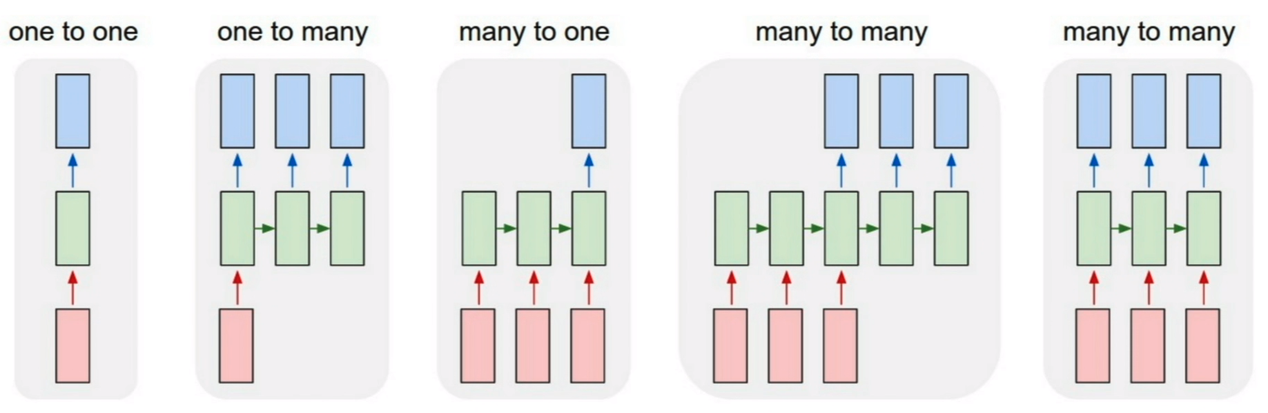
different types of problems
Vanilla Recurrent Neural Network
vanilla RNN
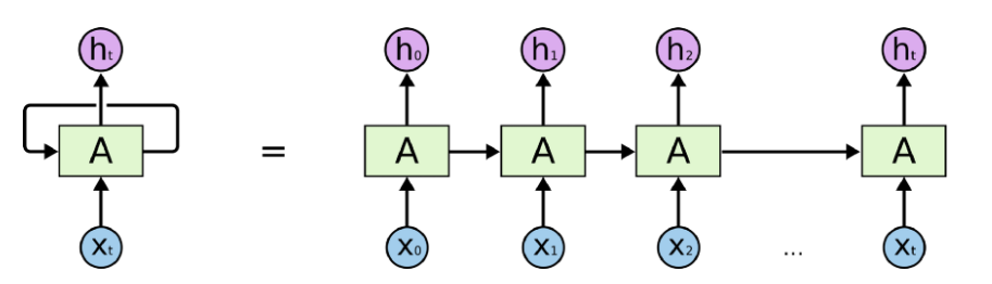
The graph above is an abstract representation of vanilla RNN. The formula is as below:
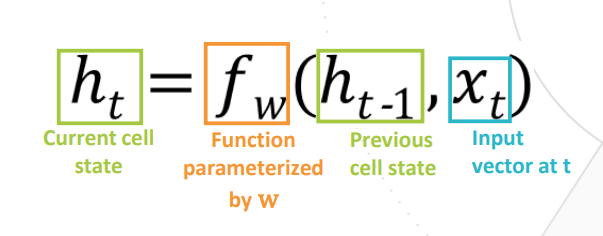
Two notes are important there. First, the hidden layer called RNN cell has several cell state, denoted by h, and the current cell state depends on the last cell state and the input at that current time step. In other words, the hidden layer involves a loop whose current input are last output and current time step.
Second, the function and its parameters remain the same at every time step.
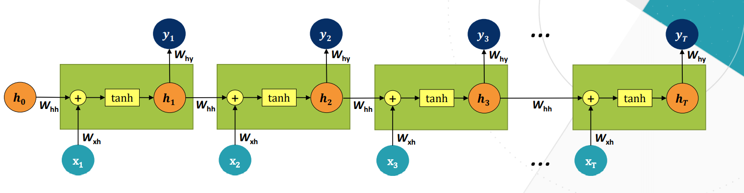
We can view its unfolded presentation in which the function is tanh, to better understand how the data is processed.
Vanishing Gradients and Exploding Gradients
As we know, the way in CNN to update the weights is back propagation. Back propagation is a way to use gradient descent to update the weights, so that the loss can go down. In RNN we use a method called back propagation through time which will multiply the same factor when computing gradients. If this factor is smaller than 1, the value will come to 0; if greater than 1, this value will become big. That’s why vanilla RNN cannot preserve long-term dependencies and why it is not considered in real problem.
LSTM
Long Short Term Memory is special kind of RNN, which is capable of learning long-term dependencies. They have the same chain-like structure like vanilla RNN and it is to change the way RNN cells managing information and gradient flow to avoid vanishing gradient problem.
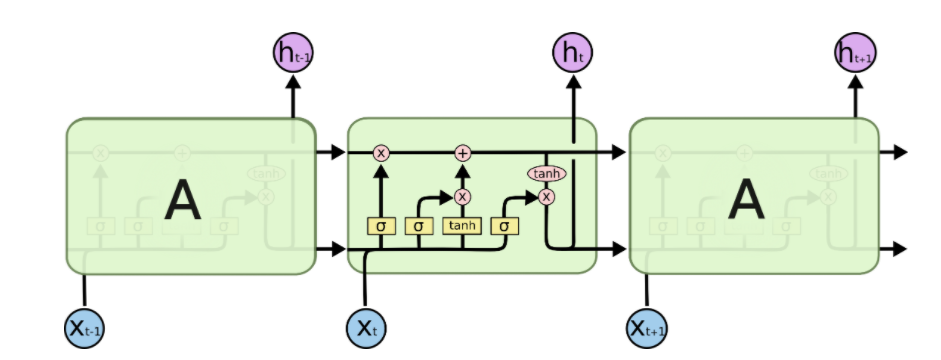
LSTM structure
The additional elements in LSTM, compared to vanilla RNN, are four gates and the core cell state. This cell state, as shown on the graph below, is designed to fight vanishing gradient problem and to track long-term dependencies like the memory. The hidden state that is used to make decision over short-term information is the same as in vanilla RNN.
The four yellow rectangles are the four gates to filter information for the cell state. They are:
Forget gate
to decide what information should we forget or keep from previous states
Input gate
to control which values will be written to current cell
Input modulation gate
to decide how much to write to current cell, which can be considered as a sub-gate of input gate
Output gate
to control the Output to cell state
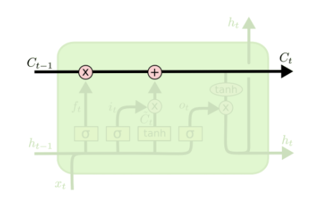
LSTM structure
Response to vanishing gradient
LSTM use BFTT method and the gradient of core cell state to update weights. However, the gradient value can be constrained by the forget gate and by the addition operation in calculation. This post have a detailed explanation how it is realized. Like what the author says, “It is the presence of the forget gate’s vector of activations in the gradient term along with additive structure which allows the LSTM to find such a parameter update at any time step[4]”.
RNN applications
RNN has various application especially in language. The tasks include text generation, machine translation etc. In the domain of image, it has application in image captioning, visual question answer, etc.
Attention in RNN
By definition, attention is the ability to decide what to focus on, to be selective about what you are looking at or thinking about. Attention is particularly useful when learning.
A natural question is: an we deploy similar attention mechanisms to help RNN to focus on specific parts of data ?
implicit attention & explicit attention
Implicit attention is quantifying what is the sensitivity of an output to inputs. DNN are huge parametric system so they all have implicit attention by nature. To assess it, we can use sequential Jacobian.
However, we need to model an attention mechanism that is more close to human’s attention, which is called explicit attention. Its advantages is that the computation time will be reduced, that the sequence will be simplified and that we can understand what RNN is concentrating on.
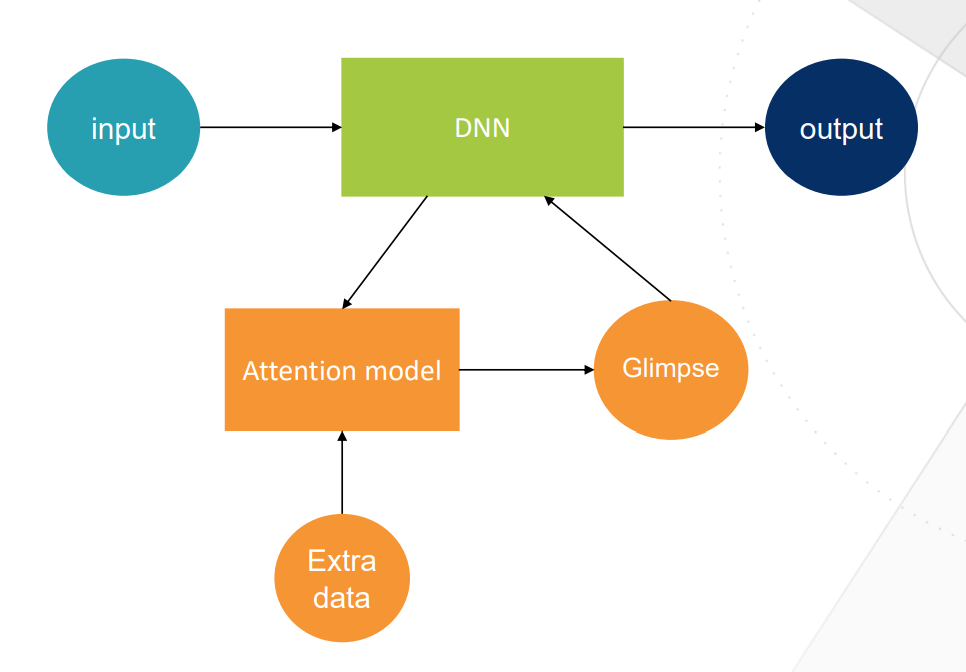
| An attention mechanism can be integrated into Deep Neural Network as the graph above. Attention models are defined by a probability distribution over glimpses: P(g | a). According to the function defining the probability distribution, attention models can be divided into two groups: hard attention models(by RL) and soft attention models(by gradient descent). |
application
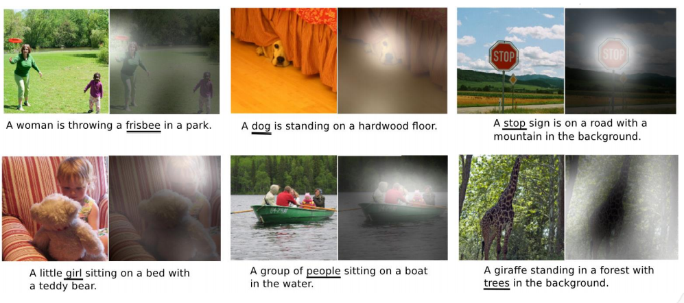
Attention mechanism can be applied in many field including images and language processing. Let us take example in image captioning. In the image below, we can use attention to gain intuition of what model sees.
Lab
The objective of this laboratory is to implement a model for image captioning, with teacher’s guide. We use the subset of dataset Common Object in COntext (COCO). Captions are provided for the training and validation data. We need to train the model and generate captions for the test data. The link to the code can be found here.
For the preprocessing part I followed the code of teacher by watching the recording. In general, an json file contains all of the captions should be split and make up a dictionary. Each word should reference to an index in this dictionary to serve as input of deep neural network model. The image below is an example with its captions.
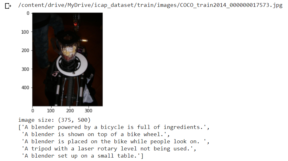
Afterwards, all the images should be preprocessed to be able to fit into the model. We can use Keras’s preprocessing API to achieve it. To define the model, we will use Transfer Learning method. It is a technique of using trained model to be the initial part of our model. InceptionV3 will be used here.
The next step is to implement the part of preparation of data. Normally, the input should be like this:
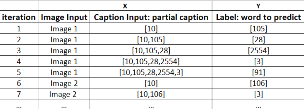
The label of current state should be the next word, and the features should be X1, the features of image, and X2, the index of words in captions.
What I implemented is as below: the first function is to get the full path will filename. In the second function, the three list are created. Each time it will get the n words in caption, and put n+1 word as label.
# from filename to ID
def filename_fullpath(name,subset):
  tmp = name.replace('COCO_train2014_', '', 1)
  id = int(tmp[:-4])
  path = getPaths(id, subset)[0]
  return path

# get inputs X and labels Y
def create_sequences(features, captions_full, subset):
  X1, X2, y =[],[],[]

  for key in features.keys():


    # path for an image in subset
    path = filename_fullpath(key, subset)

    # all the captions of this image
    captions = captions_full[path]

    # each caption of this image
    for caption in captions:
      clean = cleanCaption(caption)

      # list of all the words in this sentence
      words = clean.split(' ')
      for i in range(len(words) - 1):
        if words[i] in wordToIndexMapping:
          tmp = []
          for j in range(i):
            #tmp.append(words[j])
            if words[j] in wordToIndexMapping:
              tmp.append(wordToIndexMapping[words[j]])
          if len(tmp) != 0:
            X2.append(tmp)
            X1.append(features[key])
            #y.append(words[i])
            y.append(wordToIndexMapping[words[i]])

  return X1, X2, y
This part work well, as we see the log of first 20 items: each y is the next work of list X.
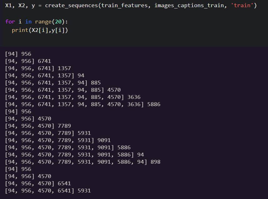
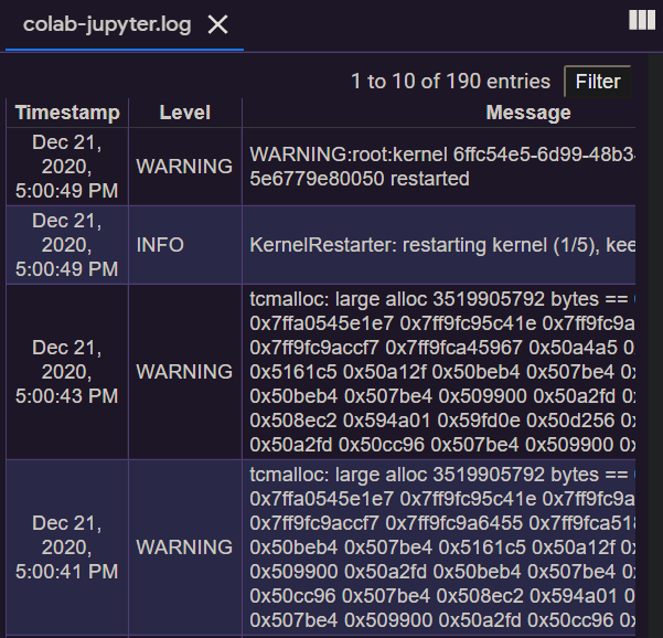
The next step it to feed the inputs into model. The part I fail after several times. I have problems on type of input and also in memory overflow. Even I try with small dataset, changing the type as float, it is the same. At last I stop at this step.
### Train the model on a small training dataset ###
X1 = np.array(X1).astype('float32')
X2 = np.array(X2).astype('int')

y = np.array(y).astype('int')

x1 = X1[:20]
x2 = X2[:20]
y_mini = y[:20]
print(len(x1))

model.fit([x1, x2],y, epochs=20, verbose=2)
References
[1].Vanilla Recurrent Neural Network [2].introduction to RNN [3].LSTM introduction [4].How LSTM networks solve the problem of vanishing gradients